
MODIS has 20 Reflective Bands (Bands 1-19, and Bands 26), with wavelengths ranging from 0.41 to 2.1 micrometers (microns) and a ground resolution of 250m, 500m, or 1km (band dependent).
Key Uses of the MODIS Reflective Bands
| BAND | |
|---|---|
| Absolute Land Cover Transformation | 1 |
| Aerosol Properties | 15 ,16 |
| Atmosphere | 13h, 13l |
| Atmospheric Properties | 16, 17, 18, 19 |
| Chlorophyll | 8, 9, 10, 11 |
| Chlorophyll Fluorescence | 14h, 14l |
| Cloud Fraction (Thin Cirrus) | 26 |
| Cloud Properties | 7, 17, 18, 19 |
| Cloud Amount | 2 |
| Green Vegetation | 4 |
| Land Properties | 7 |
| Leaf/Canopy Differences | 5 |
| Sediments | 12, 13h, 13l |
| Snow/Cloud Differences | 6 |
| Soil/Vegetation Differences | 3 |
| Troposhere Temperature | 26 |
| Vegetation Chlorophyll | 1 |
| Vegetation Land Cover Transformation | 2 |
L1B Reflective Calibration
The MODIS reflective calibration algorithm is designed to determine the at-aperture spectral radiance of the Earth scene and the bidirectional reflectance of the Earth scene with their respective associated uncertainties. Level 1A data is Earth-located raw sensor digital numbers and Level 1B data is Earth-located, calibrated data in physical units.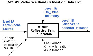
The BLUE print (upper half of figure) denotes parameters which change every scan.
The BLACK print (lower half of figure) denotes periodic or pre-launch determined parameters.
The Solar Diffuser, SpectroRadiometric Calibration Assembly (SRCA) and Space View are used periodically to determine calibration coefficients for the reflective bands. The Space View is used every scan along with the periodic calibration results to calibrate the reflective bands. The on-orbit reflective band calibration is a one-point method adjusted by data from a two-point periodic method to fit a linear detector response.
Reflective Solar Band (RSB) Calibration
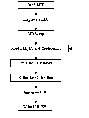
The following figure is a simplified RSB L1B flow diagram.
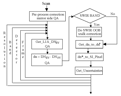
The major steps in the RSB calibration are:
- Preprocess the L1A telemetry and onboard calibrator (OBC) data, retrieve the required LUT files and develop time dependent gain factors.
- Retrieve L1A Earth view (EV) DN (digital number) and subtract the average (50 samples per scan) space view (SV) background

- For the SWIR Bands (5-7 and 26), apply the thermal leak correction. (The thermal leak is caused by energy from near 5.5 micrometers striking the SWIR detectors. The radiance from Band 28 (7334 nm) is used as a surrogate for the leak. Therefore, the thermal bands must be calibrated prior to the reflected bands as shown in the following figure:)
 MODIS Level 1B Algorithm
The Earth-view portion of a scan from one side of the MODIS double-sided scan mirror sweeps out an area 10 pixels along- track by 1354 pixels (or frames) cross-track. At nadir, these pixels are 1X1 kilometer. A pixel advance (1 km) cross-track is a frame. A frame includes 10 pixels (along-track) from each of the 36 bands. Each pixel of the two 250 meter bands has 16 sub-frames (digital samples) and each pixel of the five 500 meter bands has 4 sub-frames. In addition, Bands 13 and 14 output both high- and low-gain values. Each frame therefore consists of 830 digital numbers (DNs). Each value is indexed by band, detector, sub-frame and mirror-side (BDSM) and each is calibrated independently.
The L1B software is divided into two major modules. One applies the radiometric calibration and develops uncertainty indices for the 20 Reflective Solar Bands (RSBs) (Bands 1-19 and 26) and the second does the same for the 16 Thermal Emissive Bands (TEBs) (Bands 20-25 and 27-36). The radiometric calibration and uncertainty procedures are described in the following sections.
At any given time, there are two current versions of the L1B software and the numerous LUTs in order to accommodate minor differences in the Terra and Aqua sensors. Changes in both sets of software and updates of the LUTs are carefully tracked and archived so as to enable data reprocessing.
- Apply temperature and time-dependent response versus scan angle (RVS(t)) corrections.

where kInst is the instrument temperature correction coefficient determined pre- launch,
TInst is the instrument temperature and
Tref is the reference temperature used to determine kInst. - Compute the reflectance factor
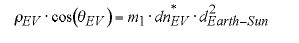
m1 = Reflectance scaling coefficients determined offline from SD/SDSM calibration
dn*EV = MODIS detector’s "corrected" digital number (see E)
dEarth-Sun = Normalized Earth-Sun distance (calculated from the data granule time) - Convert the reflectance factor to scaled integer (SI) (see section below).
-
Calculate the RSS uncertainty for each sample and convert to an uncertainty index (UI) (see section below).
Uncertainty Index
For each pixel, the Uncertainty Index (UI), with a range of 0-15, is computed online using the following:
UI = scaling_factor[B]•ln(sEV/specified_uncertainty[B])
The band dependent scaling factors and specified uncertainty values come from LUT inputs. The RSS uncertainty, sEV (in percent), is computed dynamically.
UI utilizes the first four bits of an 8-bit unsigned integer, which yields a range of 0-15.
Scaled Integer Conversion
The TEB radiance values, LEV (W/m2/µm/sr), are scaled to an integer range of 0-32767 over the LUT-supplied dynamic range of Lmin to Lmax using:
SI(BDF)=32767*(LEV(BDF)- Lmin(BDF))/(Lmax(B)- Lmin(B))
LEV (a 32-bit floating-point number) is scaled to a valid integer of 0 to 32767, using 15 bits of a 16-bit integer number. SIs greater than 32767 are reserved for invalid data.
The LUT-fuished values of Lmin and Lmax are indexed by band only.
The RSB reflectance factors are scaled in a similar manner.